Algomia Solver

Combinatorial optimization has proved time and again, to be an extremely useful method for deriving better decisions, whenever scarce and constrained resources have to be allocated. Typical areas of industrial use-cases include transportation, logistics, healthcare, finance, technology, defense, and more. A common problem is combinatorial explosion at growing problem-sizes, which limits the scalability of algorithms. Given the usefulness of the combinatorial optimization approach, the need for large-scale solvers becomes evident.

This page shows our design and implementation of our a flow-based solver for large-scale and real-world combinatorial optimization.

Our main design goals and decisions have been:

1. We require that the solver is applicable to a broad variety (if not all) of combinatorial optimization problems, with reasonable modeling efforts. Our answer to this is to formulate any combinatorial optimization problem in terms of SET CONSTRAINED FLOW, which extends network flows with additional edge-set constraints.
2. Many real-world use-cases have locality and globality properties, that shall be supported in the modeling: There is a clear separation between groups of constraints that link resources at a narrow perspective, e.g., precendence requirements for tasks, and groups of constraints that have to hold at a high level view, e.g., task coverage requirements. In our approach, local constraints are mostly captured in a network, while the global constraints are treated with edge-set constraints.
3. At the same time, we want to provide strong guardrails in modeling, by only allowing a small number of types of constraints.
4. The solver has to scale “out of the box”. We chose to implement a long-known, proven method for solving large-scale linear programs: column generation. The approach iterates between solving master- and pricing-problems. We solve the pricing- problems parallel, and will implement GPU support soon.
5. We seek to have guarantees on the quality of the solutions found by the solver. Comparing the objective-value of the solution of the solver with the linear programming lower bound, determined by column generation, achieves this goal in a well-known manner.
6. Expert users shall be able to configure the solver, in order to fine-tune it towards their use-cases. We argue that our modular architecture, see below, yields this objective. Our implementations of the modules that have been tested and yield proven value.
7. The software shall be accessible easily, even if sophisticated features, like GPU-acceleration (once supported), are in place. It was straightforward to make the solver available through a REST API, which hides the technical deployment details from a user.

Our algorithm solves a combinatorial optimization problem called SET CONSTRAINED FLOW directly, by employing the column generation method in a modular software architecture. In this section, we summarize our approach.

2.1 Problem Formulation

The problem SET CONSTRAINED FLOW is defined as follows: We are given a directed graph \( G = (V, E) \) on n vertices and m edges, and a family \( S = \{S_1, \ldots, S_k \} \) of k set constraints, where the element \( S_i = (E_i, \ell_i, u_i) \) defines some set \( E_i \subseteq E \) and two numbers \( \ell_i \leq u_i \). Each vertex \( v \in V \) is given by a pair \( v = (i_v, b_v) \), where \( i_v \in \mathbb{N} \) is a unique identifier, and \( b_v \in \mathbb{R} \), the balance of v. A vertex v is called a source if \( b_v > 0 \) and a sink if \( b_v < 0 \). Each edge \( e \in E \) is given by a tuple \( e = (i_e, s_e, t_e, c_e, w_e, d_e) \), where \( i_e \in \mathbb{N} \) is a unique identifier, \( s_e \in V \) is the source, \( t_e \in V \) is the target, \( c_e \in \mathbb{R} \) is the cost, \( w_e \) is the weight, and finally \( d_e \in \{\mathbb{B}, \mathbb{Z}, \mathbb{R} \} \) is the domain of e. For each edge e, there is a variable \( x_e \in d_e \), i.e., in the domain given by the edge. Define the vector \( \mathbf{x} = (x_e : e \in E) \) and its cost by \( \textnormal{cost}(\mathbf{x}) = \sum_{e \in E} c_e x_e \). The optimization problem is:

Here, (1) is the objective function, (2) are the balance constraints, (3) are the upper constraints, and (4) are the lower constraints. \( E^-_v \) and \( E^+_v \) denote the incoming and outgoing edges of vertex v. SET CONSTRAINED FLOW is said to be in canonical form, if there is a singleton constraint \( S_i \in S \) with \( E_i = \{e\} \), \( l_i = 0 \), and \( w_e > 0 \) for each \( e \in E \). In that case, we identify i and e, and the edge e has a capacity \( k_e = u_e / w_e \). Observe that MINIMUM COST FLOW and hence also SHORTEST PATH are direct special cases of SET CONSTRAINED FLOW in canonical form.

2.2 Modular Software Architecture

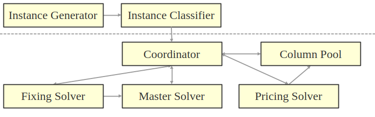
The initial module is the instance generator, which is a framework that help to transform the input of some given use-case into an instance of SET CONSTRAINED FLOW. The user simply has to define the inter-dependencies between the objects of the use-case. The actual graph generation is taken care of by the module, by making use of parallelization to speed up the process. Finally, the user needs to specify the set constraints to complete the definition of the instance. Given that, the instance classifier detects properties that will be exploited in the subsequent modules and hence affects the overall configuration of the optimizer.

The main module of the solver is the coordinator: It instructs the behaviour of the remaining modules, observes if a terminating solution has been found or if time-limits have been exceeded. Following the column generation approach, the constraints of the instance are split into local- and global constraints, respectively. The master solver hosts the global constraints and always solves some given linear program. The corresponding dual solution yields reduced cost coefficients on the edges, which are reported to the pricing solver by the coordinator. The pricing solver solves the subproblem, which is given by the graph, the local singleton constraints, and the vertex-balances. In many cases, these problems are simply SHORTEST PATH problems of some variety (and determined by the instance classifier). The pricing solver is responsible for most of the speed and scalability of our approach: SHORTEST PATH can be solved in low order polynomial time and a large number of paths can be generated in parallel. The paths are reported to the column pool, deciding which ones to keep and which ones to discard. The remaining columns are finally added to the linear program to be solved by the master solver. Finally, the fixing solver decides which variables or constraints in the linear program are rounded, frozen, or released.